Wondering about that itinerary's reliability?

We're predicting misconnection and delay chances—and they're readily accessible.

If you haven’t booked your flights for holiday travel yet, we might be able to reward your procrastination. Or at least take the sting out of the higher prices you’re predicted to pay.

Because that’s the thing: most OTA’s and aggregators prognosticate about the direction of prices (even if you ignore it). And increasingly, price forecasts are presented alongside emissions estimates. So you’re guided towards the most sustainable option with the most economical timing. But what about the most reliable option? Frequent fliers can recognize a red flag in a routing, though a behavioral economist would wince at the most well-tuned mental model of the national airspace system. (To say nothing of the infrequent flier.)

Layovers and it’s-gonna-be-tight arrival times can be a gamble; we think travelers should be better informed about the odds. To that end, we’ve developed an algorithm that answers how likely is an itinerary to get you there when advertised. More technically, we built a density network. It’s an AI architecture that taps the power of neural networks to estimate the range of possible outcomes—and the likelihoods within that range.

In our case, we’re aiming it at the distribution of delays, a problem where uncertainty abounds even with a prediction horizon of a couple hours. Is your aircraft going to require an unplanned tire change? Is your pilot going to sleep through their alarm? Your catering truck? Could get in a fender bender. Passengers? Pesky things are one airport beer too many away from having to be deplaned. Plus a ripple effect. And that’s when you have a reasonably good idea what the weather is doing and where your plane is coming from!

At a months-ahead horizon—when weather forecasts are more coarse and less skillful—it’s all the more important to frame flight outcomes in terms of chances, not single estimates. Within a practical range of over-blocked, tailwind-aided 60 minutes early to might-as-well be cancelled 24 hours late, no exact delay minute is all that likely. While it might not feel like it, arrival delays gravitate towards negative values (read: early arrival); but even within this relative peak, the single most likely outcome (10 minutes early) only happens about 2.5% of the time.

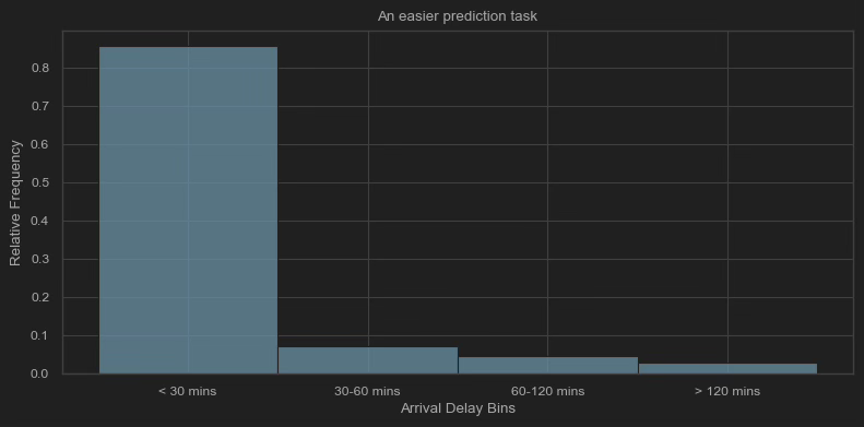
One approach to dealing with this uncertainty is binning several delay minutes together (see below), rather than treating each delay minute as its own unique possibility (like the above chart does). It makes for an easier prediction task: you’d be trying tease apart fewer outcomes with higher likelihoods. If you bin arrival delays into less than 30 minutes, between 30 and 60 minutes, between 60 and 120 minutes and greater that 120 minutes—like Amadeus does—the bin with the lowest frequency (120+ minutes) is more probable than our most probable single value (-10 minutes exactly).

But easier for the forecaster doesn’t mean more usable for the traveler. The bins mask some material differences. Maybe you can absorb as much as 90 minutes delay, but beyond that you’ll miss the start of the meeting. Or even more consequentially, maybe your 65-minute layover is doable with a 30 minute delay but hopeless with a 55 minute delay.

Our density network is well suited for capturing this uncertainty with much higher resolution, i.e. distinguishing between the 30 and 55 minute delay. Let’s see what that looks like.

Get chances

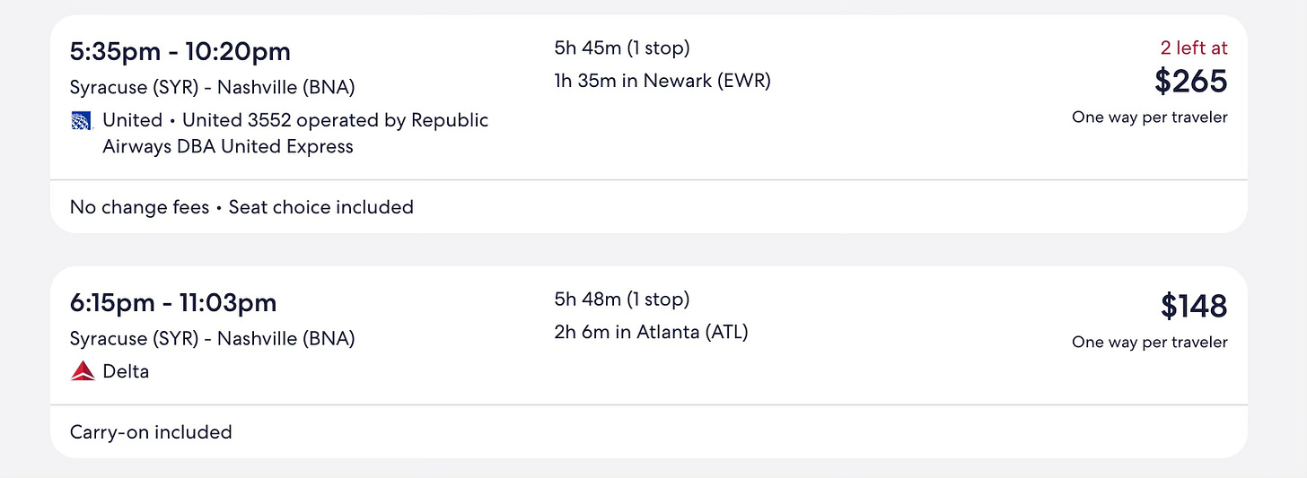
Consider somebody flying from Syracuse (SYR) to Nashville (BNA) on the Tuesday before Thanksgiving. They’ve found two options with similar travel times that allow for a close-to-full day of work.

They’re a frequent enough flyer to vaguely know EWR’s reputation, but 95 minutes seems generous? And they’re seriously averse to getting in the door after midnight—so the 40-minute earlier arrival should provide a better chance to be in the Uber by 11:45 p.m., right? They switch from their Expedia tab to Aerology’s forecast, input the details for the via EWR option and hit “Get chances.”

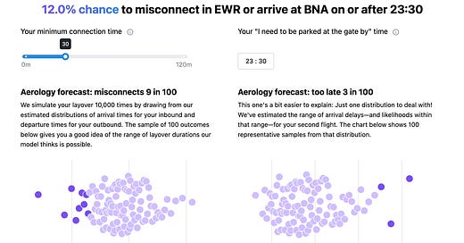
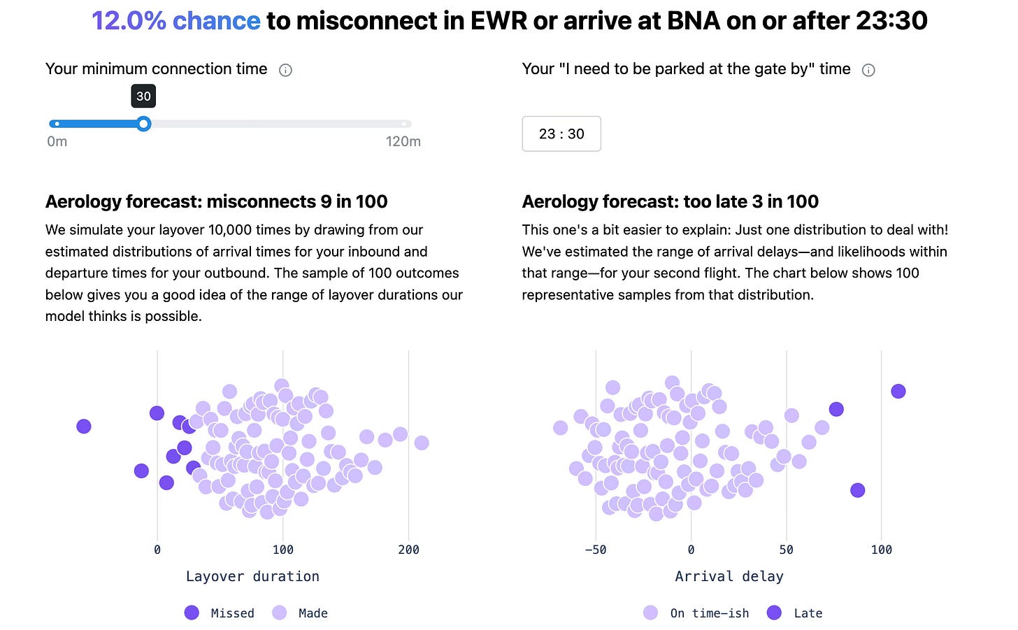
Under-the-hood, we’ll estimate the distribution of arrival delays for the SYR-EWR flight and the distribution of departure delays for EWR-BNA, then randomly sample from those distributions. That first sample might “draw” an arrival delay of -6 minutes and a departure delay of 2 minutes; given the scheduled layover of 95 minutes, that first simulation nets out to 103 minutes of available connecting time. Then we do it 9,999 more times and visualize 100 representative outcomes. By default, simulations that provide less than 30 minutes to connect are considered missed and, in the case of our BNA-bound traveler, we forecast they’ll be left with an insufficient layover duration about 9% of the time¹.

And while a missed connection is a good bet to screw up your schedule, there’s likely some amount of delay to your originally scheduled arrival that you can’t afford. For this reason, we’ll also sample from our estimated distribution of arrival delays to your second leg (EWR-BNA, in this setup). Here, by default, we’ll assume you can only absorb about an hour of delay; for our BNA-bound, the default is about right with respect to getting in the door by midnight.

Because we don’t need to net out the layover or a second delay for this part of our forecast, you can also use it as a workaround to one our design decisions. To maximize applicability, we’ve geared this initial version towards one stop itineraries; it may be a bit hack-y, but if you want to glean disruption chances for a non-stop itinerary, you can treat the second leg as your non-stop (i.e. use the layover airport as your origin). You’ll need to invent a first leg and, depending on the fictional first leg, the misconnection and headline chances should only be referenced for a laugh. But because our forecast of the second leg’s arrival delay is independent from the first leg, the too late forecast is representative of your non-stop’s chances.

That last sentence is an important distinction. The too late forecast does not ask what are the chances I arrive by this time, given that I make my connection. It provides the chances that the flight arrives by that time—whether you’re on it or not. It’s also why the headline number (12% for our SYR-EWR-BNA option) may not equal the sum of misconnects and too late: there’s some too-late outcomes that could have still resulted in a misconnect. The headline asks what are the chances that I misconnect or arrive too late; it could also be framed as what are the chances I make my connection and arrive on time-ish.

To contextualize that 12% disruption probability, it’s about the same as parents having three children of the same sex. But we think our forecasts are best employed in bunches. It provides better context than thinking through the boy/girl mix of your friends and family. So our BNA-bound traveler opens another tab (… our design road map takes note), inputs the details for the via-ATL option, adjusts the too-late threshold to 11:30 p.m., and finds something like an 8.1% chance to mis-connect or arrive too late. Despite a scheduled arrival time that’s 40 minutes earlier, the over-EWR option is nearly 50% more likely to leave our hypothetical traveler short of their door by midnight.

🤨 And why should I trust you guys?

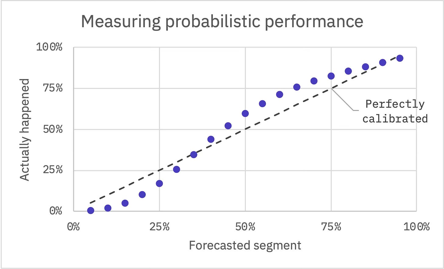
It’s a fair question. A single prediction can be hard to judge on its own, especially when it’s of the percentages variety. For that reason, we took great care to create a test set numbering more than 4.5 million flights that we can use to evaluate our models’ performance. Because we’ve approached this problem probabilistically (i.e. we’re not making a single estimate but rather estimating likelihoods within a range of possible outcomes), one of our most important metrics is the degree to which forecasts are well-calibrated. If they are well-calibrated, it means an outcome actually occurs at roughly the same frequency as we predicted.

For each flight in our test set, we can segment our predicted distribution. For example, calculate the minute where we’d say there’s a 35% chance that actual delay will be less than or equal to that threshold—then we should find, with a well-calibrated forecast, that actual delay falls into this segment about 35% of the time. In the case of the predicted segment where we’d say there’s a 35% chance for delay less than or equal to that minute, 34.5% of actual values fell within the segment.

We tend to be a bit over-confident at lower probabilities, which is to say these events actually happen less often than we forecast. For the segment where we’d predict 15% of delays will fall in, just 5% actually do. Oppositely, we exhibit some under-confidence for probabilities higher than 50%. But, overall, we think our forecasts performed quite well—certainly well enough to underpin an MVP. It’s an open beta, so no credentials required and feedback welcome!

1. Because we’re randomly sampling, your 10,000 simulations will be slightly different from our 10,000 simulations; and successive forecasts for the same set-up will likewise differ slightly.