

A climate tech pivot: carbon removal via airship
A climate tech pivot: carbon removal via airship
How to use 43% more solar resource per square meter than the Mojave

Executive Summary
In a radical departure from previous Aerology newsletters, this post explores—and I believe substantiates—the technical and economic viability of carbon removal via airship. Rather than using fans to push air across a filter, the filter is propelled through the air (with less energy required). An airship’s mobility allows for solar resource seeking and reduces land consumption; decoupling from utilities also reduces process emissions, thus reducing our net removed cost. An “empty” airship (i.e. without filter) is estimated to cost $31k with a lifetime of 8 years, during which time it will autonomously capture 948 tons; scaled to 8,700 airships, we could remove 1 Mt per year. Presumably operating in an oceanic environment situates these micro-plants atop a strong carbon sink (and abundant offshore energy): inter-platform drones can dispatch captured CO2 to sea surface platforms for storage. Even when accounting for higher post-airship costs, the proposed net removed cost ($171/ton) is 25% lower than a grid-tied, natural gas-supplied plant.
Having graduated to technical founder at an AI startup, I figured I’d bust myself back to non-technical founder at hard tech startup. See, the threshold of Aerology’s runway has come into view and the flight disruption mitigation idea wasn’t generating enough lift. Maybe there’s a post-mortem coming in a future post; and there’s several prototypes that I believe are worth building upon and for which I’d like to find a home. But with the last few feet of runway, I’m going to [beat this metaphor to death and] try a radically different configuration. To that end, this pivot is probably just as fairly described as a Hail Mary (or an idea for a new startup): but if the below resonates with you, I’m looking for investors, builders and investors at tim@aerology.ai!
The idea was borne from wondering if carbon could be captured from the exhaust plumes of aircraft, à la point-source capture from industrial flue gas streams. Minimizing separation and maintaining stable, intra-wake flight would create some incremental regulatory and engineering burden1, so I needed to reduce this initial idea to something more minimally viable—to something that looks like direct air capture.
What is direct air capture?
Direct air capture (DAC) extracts CO2 directly from ambient air2. Fans push air through large contactors, wherein CO2 is adsorbed by a capture agent (i.e. sorbent). CO2 is periodically desorbed (i.e. separated from the capture agent) using heat then compressed for transportation.
Relatively dilute CO2 concentrations in ambient air translate to higher energy requirements compared to point-source capture. This energy intensity not only directly inflates costs, but can materially depress net CO2 removal if the power source produces emissions itself.
I’ve oriented around an autonomous airship solution, inspired by Alphabet’s balloon-based internet moonshot (and the wealth of information they shared). Before we dig into the techno- part of this analysis, however, let’s level-set on the economic part.
Create a 2030 economic base case: grid-tied, nat gas-supplied plant
I relied heavily on this paper for costing (referred to as McQueen et al 2020 when it might be unclear what paper I’m using). Not only is the “plant modification” approach extensible to our concept but, reassuringly, its lead author also co-founded an especially innovative direct air capture company. The first order of business was to update the paper’s base case to a 2030 horizon, which is a common milestone in literature and would represent a reasonable target for starting to scale our technology.
I’ll liberally use footnotes to explain assumptions throughout this analysis. Given the length of this post and easier footnote navigation, I’d suggest switching to the web (or the Substack app) if you’re reading this in email form. For those looking for something more skim-able, I’ve tried to bold snippets herein to create a shorter, coherent-ish narrative; I’ve also forgone some creativity in section headings to hopefully make it easier to find what you’re looking for. Additional details can be found in this notebook (it’s written in Python, though it’s not especially Pythonic).
Creating the 2030 base case for conventional DAC entailed:
Splitting out transportation (trucking, in the case of the paper) from compression CapEx3.
Forecast 2030 contactor CapEx (i.e. sorbent and sorbent supporting structure) and storage OpEx costs, using improvement rates4 from this paper’s supplement. McQueen et al (2020) analyzed a solid sorbent system (versus liquid), which is favored for its lower temperature requirements; solid sorbent DAC also promises better modularity and was selected for this analysis.
Forecast 2030 steam OpEx costs using an assumed thermal energy requirement5 of 3.4 GJ/ton (down from 8 GJ/ton employed in McQueen et al 2020).
Update 2030 maintenance and labor OpEx, which are a fixed fraction of CapEx.
Adding storage OpEx, so that cost reflects “to-grave,” not “to-gate” ($11/ton flat fee lifted from McQueen et al 2020 supplement); forecasted improvement at a 1.3% rate (Subterranean or submarine CO2 storage domain).
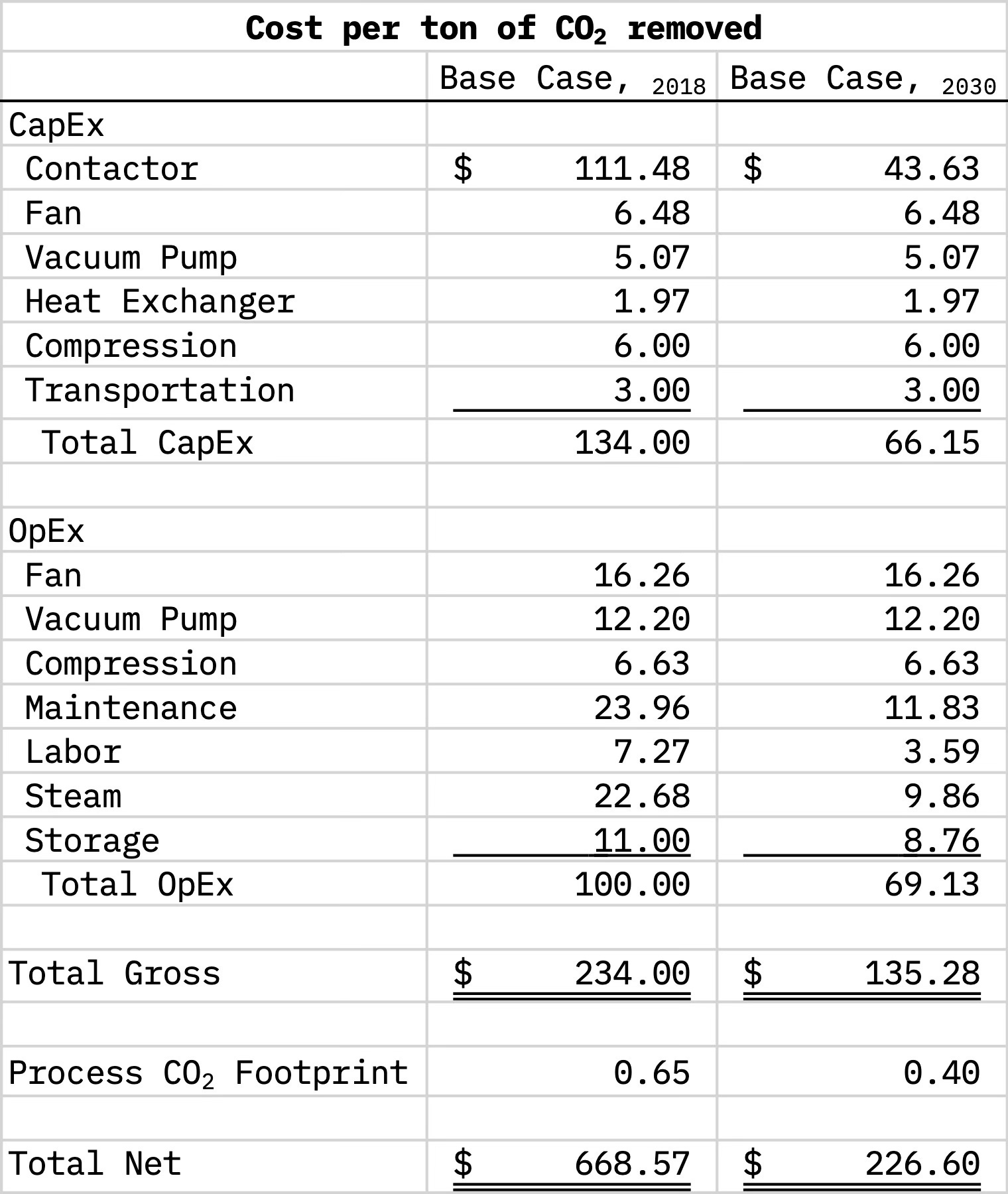
This yields an estimated 2030 baseline cost of $135.28 removed CO2 (comprised of $66.15 in CapEx, $69.13 in OpEx), down from the paper’s 2018 estimate of $234. From now on, we’ll refer to this amount—the sum of CapEx and OpEx—as gross cost. This gross prefix indicates that the CO2 emitted during the process of carbon removal has not yet been netted out. Process emissions are mostly6 a product of energy consumption associated with operating fans and pumps (i.e. electrical) as well as regenerating the sorbent (thermal). McQueen et al (2020) sized this footprint at 0.65 tons CO2 emitted/ton removed for their 2018 base case, from which we derived our above 2030 baseline.
These conventional scenarios assume thermal energy is furnished from steam supplied by natural gas while the fans and pumps are powered by the electrical grid. As a result of reduced thermal energy requirements and a cleaner grid, I estimate our 2030 baseline emits 0.40 ton CO2/ton removed7. Notably, this assumes that grid intensity continues to improve at a linear rate consistent with the last five years (from 373.4 g CO2 emitted/kWh consumed in 2024 to 290.7 by 2030).
And that may not be a good assumption.
Data centers are putting new demand on the grid—while the US falters on permitting and interconnection reform. (To say nothing of a posture towards nuclear than can be described, at best, as waffling.)
And grid intensity—along with thermal requirements—is critical to the viability of DAC because these emissions inflate the cost per ton CO2 removed. The earlier-calculated $133 doesn’t actually remove 1 ton of CO2; it removes 0.60 tons CO2, less the 0.40 tons emitted. And it actually takes the removal of 1.67 tons, at a net cost of $226.60/ton, to say you’ve removed 1 ton of CO2 from the atmosphere. This net cost can be calculated as:
where x is CO2 emitted/CO2 removed footprint.
So what might one do to decouple DAC economics from grid intensities and relatively-clean-but-still-combustion natural gas? They’d go off-grid.
Model solar resource for irradiance-seeking airship (🖕, NIMBYs)
That might mean integrating with a dedicated solar array—Terraform Industries is doing some impossibly improbably cool things in this space that includes DAC. But grid-tied, natural gas-supplied DAC is not without land usage concerns. And an accompanying solar farm would increase land use requirements by 5-6 times. A solar-powered DAC plant would require an area approximately equal to 1 sq. km, or about 45 Manhattan8 blocks, to remove 1 Mt (megaton) CO2. IEA’s Net Zero roadmap pencils DAC in for 75 Mt/year capacity by 2030 and 630 Mt/year by 2050: if entirely solar-powered, that requires an areal footprint greater than Manhattan (59 sq. km) and approximately equal to the San Francisco Peninsula north of Menlo Park, respectively.
Frustratingly, it’s not so much a matter of land availability. Arizona alone has nearly 6,500 sq. km of suitable9 land. It’s the NIMBYs. And their faux environmentalist conspirators. They’ll aim to turn it into a legal slog. With just 4.7 Mt capacity in the 2030 pipeline that’s under construction or in advanced development, slog is not the target velocity. The regulatory burden of air navigation service providers seems like a bargain by comparison.
Our micro plant’s mobility not only detangles us from the NIMBYs but, more importantly, also enables solar resource-seeking. (It also mitigates some marginal risk about CO2 depletion10.) The vehicle can consistently operate in the longest, clearest days; and operating at an altitude of 5.4 km11, just below the floor of Class A airspace, further amplifies solar irradiance.
To determine the solar resource available to such a vehicle, I built a reinforcement learning algorithm12 that trained on all-sky direct normal irradiance (DNI) estimates from NASA POWER. The result—let’s call it modestly optimized, possibly conservative13—is an estimated 11.62 kWh per square meter per day. An ideally sited location in the US (like Sunfair, CA in the Mojave Desert) looks to receive 8.15 kWh per square meter per day; the average location in the US receives 5.30 kWh per square meter per day. So we can harness 43% more solar resource than even the most irradiated surface in the US (and more than double that of the average site in the US).
Now, we don’t get to utilize the entirety of this 11.6 kWh: a solar technology’s efficiency is the energy harvested as a percentage of the available resource. Probably-pictured solar photovoltaic (PV) will generate electricity. Lesser known—but more efficient—concentrated solar-thermal power (CSP, which uses mirrors to focus sunlight on heat transfer fluid) will generate heat. Let’s treat PV first.
Determine non-payload specifications
Commercially available, state-of-the-art panels report an efficiency of 22.8%, but efficiency varies directly with irradiance and standard test conditions14 assume more irradiance than even our optimized level. I also want to account for continued improvement in efficiencies, though applying an improvement rate linearly to model an increasing variable (especially one with a physical upper limit, like 100%) is inappropriately bullish. On today’s SOTA Efficiency x Irradiance curve, I’d expect to realize an efficiency of 20.5%; applying a logistic growth model15 to project forward to 2030 yields an estimated 24.7% PV efficiency.
What systems will this efficiency flow through to and how much energy will they require? We’ll need to estimate the needs of propulsion, onboard computers and flight control components. From this point forward, we’ll rely more heavily on the Loon Library than McQueen et al or other techno-economic assessments of [conventional] DAC approaches. The first references we’ll lift from the moonshot’s lessons relate to their Raptor vehicle, a more aerodynamically shaped balloon that was only in the prototyping phase when Loon shut down. Raptor was estimated to harvest 129 kWh/day, 30% of which was earmarked for propelling the vehicle at a speed of 5.25 m/s.
Loon’s initial versions were an un-propelled, [not-especially-aerodynamic] pumpkin-shaped balloon that exploited winds at various altitudes to navigate. They introduced propulsion and began to explore aerodynamically shaped balloons (i.e. airship) to more effectively loiter over—and quickly loop back to—areas where they were beaming internet service. Our airships wouldn’t need to station keep in the same way; there’s more navigational freedom when the target is sunlight16 and wind-based navigation would probably suffice. We do need propulsion, however, to generate the gas velocity that fans produce in conventional DAC plants. In short, we’ll propel the sorbent through the air rather than push air across the sorbent.
Helpfully, we can forfeit some of Raptor’s speed. Increasing gas velocity can improve adsorption, but only up to 3.0 m/s—so the solar panel and battery weight Loon spent getting from 3.0 to 5.25 m/s can be recouped. And because power scales with the cube of speed, reducing speed by 43% allows for a 81% reduction in power; whereas Raptor required an 38.7 kWh/day for propulsion, our airship should only require 7.2 kWh/day17. To account for the energy requirements of avionics, let’s add another 4.6 kWh/day: it’s half the daily harvest of Plover, an early, un-propelled ballon (and assumes the other half was allocated to their comms service payload, which we’re not responsible for powering).
With each m2 of solar PV panel generating 2.87 kWh/day (24.7% of the resource available to it), we’ll require 4.1 square meters to meet a daily electrical requirement of 11.85 kWh (propulsion plus avionics).
For PV, we determined how much energy the airship required; the PV panels are the power plant and integral to the airship. Concentrated solar-thermal power (CSP) is more like payload however; to size it, we need to ask how much weight is available. So let’s next outline the airship’s remaining specifications.
To that end, the next reference we’ll borrow from the Loon Library is 2,713 cubic meters: the envelope volume of Quail, their last production balloon. We’ll assume our airship has the same envelope volume, though our lower operating altitude will allow us to lift a much greater mass. Loon operated in the stratosphere, between roughly 15-20 km altitude, where a single balloon could provide internet service to an area that might otherwise require hundreds of communications towers. But this expansive service area is not free—air density in the stratosphere is around 1/10th of sea level, which demanded extremely large balloons to displace a volume of [extremely thin] air with a mass equal to the vehicle. At 5.4 km, where air density is more like three-fifths of sea level, the same envelope volume can lift a considerably greater mass. Paired with a marginal lifting benefit by way of using hydrogen, rather than helium, I estimate18 a Quail-sized envelope could lift 1,779 kg to 5.4 km.
We’ll assume Quail’s battery density was 250 Wh/kg circa 2019 (see 2:57… not my proudest citation), which would entail 16.6 kg to accommodate its storage capacity of 4.2 kWh. Plus 49.8 kg associated with Quail’s 4.6 square meters of PV, let’s say their last production ballon carried 66.4 kg for generating and storing power. I elected to ignore the weight of Loon’s comms payload—this will result in slightly overestimating our airship’s aerial systems weight and, therefore, underestimating its available payload. (Perhaps this is where we account for the weight of a possible, otherwise unconsidered heat exchanger.) That said, I estimated that Quail’s balloon, avionics, flight controls and supporting structures weighed 195 kg (its lifting capacity of 261 kg less 66.4 kg).
Battery densities are tracking for 500 Wh/kg by 2030, which would allow us to store 5.1 kWh—43% of our daily electrical requirement and proportional to Quail’s19 battery capacity:daily harvest ratio—at a weight of 10.1 kg. Add the 44.7 kg resulting from our airship’s 4.1 square meters of PV panel and we land at 54.8 kg associated with electric energy. When we deduct this electric energy weight as well as the balloon and flight systems from the lifting capacity of 1,779 kg, we find 1,530 kg available for our DAC payload. This payload will include CSP, sorbent (including supporting structure) and CO2 storage.
The mission: estimate airship’s payload and capture productivity
To determine how that available weight will be consumed by various DAC components and, ultimately, the amount of CO2 captured, we’ll return to solar resource. We had previously estimated that a square meter of PV panel would convert 24.7% of the available 11.6 kWh/day to electric energy. CSP can produce electricity, typically using the thermal energy present in the heat transfer fluid to power a turbine. But if you discharge CSP with generating electricity—i.e. you’re unconcerned about the second step’s thermal-to-electric efficiency—you’re availed relatively high solar-to-thermal efficiencies. Like we did with PV, we need to adjust for irradiance (to 67.7%) and then project forward20 to 2030, when I forecast solar-thermal efficiency will be 75%.
Each square meter of CSP will generate 8.7 kWh/day thermal energy, which is equivalent to 10.4 GJ per 330-day operating year. Given the above-estimated thermal requirement of 3.4 GJ/ton CO2 for sorbent regeneration, each square meter of CSP can produce 3.05 tons of CO2.
This square meter of CSP (mirror and frame) also weighs 22.5 kg. The sorbent and supporting structure will add another 17 kg of payload per square meter of CSP, assuming sorbent consumption improves21 to 3.71 kg/ton CO2 captured (and a 0.2 structure kg:sorbent kg ratio). Estimating the weight related to CO2 storage is complicated by operating in relatively low pressure environments—and unfortunately proves to be an unfavorable complication. If each square meter of CSP produces 3.05 tons per 330-day operating year and production occurs only during daylight hours22 (i.e. no thermal energy storage), that reduces to 14.7 g per operating minute. A 16-minute adsorption cycle, which is at the low end of the National Academy of Science’s realistic range, would produce 95 L of uncompressed CO2 per square meter of CSP at sea level; at 5.4 km altitude, the same mass of uncompressed CO2 (187 g) occupies a volume of 175 L.
This techno-economic analysis assumes compression takes place post-airship (we’ll get to that shortly), but increasingly I suspect we’d want to carry the weight23 of at least some compression. McQueen et al included 5-stage compression to 1.7 MPa (sea level pressure is 0.1 MPa) prior to transport via truck—I don’t think we’d tackle that full compression range onboard the airship, but perhaps to 0.689 MPa. That’s equivalent to 100 psi, which looks to be a common maximum pressure, and also quite close to McCollum and Ogden's 3-stage compression ratio (13.2) applied to our 0.051 MPa starting point. Split compression would forfeit some economies of scale and require heavier-duty tanks, but the same 187 g of CO2 compressed to 0.689 MPa [will possibly transition to a denser liquid state and] occupies 13 L.
With smaller per-cycle volumes (not masses!), we could more feasibly aggregate CO2 from multiple cycles prior to dispatching from the airship; and less frequent trips for these to-surface drones should, generally, permit longer trips. For now, however, we’ll assume no on-airship compression. It means we’ll have to contain relatively larger volumes of CO2, but can do so with relatively lightweight material. Recycled high-density polyethylene (R-HDPE) with a wall thickness of 2 mm was used for this analysis, though a flexible, bladder-like tank could deliver additional weight savings. I modeled a generic cylinder weighing 4.7 kg to contain the 16-minute output of one square meter of CSP: add this to the 17 kg of sorbent, 22.5 kg of mirrors and their supporting structure.
So we’ll carry 40.8 kg for each square meter of CSP. With 1,530 kg of available payload, we can accommodate the weight of 37.5 square meters of CSP. And if each square meter of CSP can capture 3.05 tons annually, our airship’s estimated productivity works out to 114.48 tons per year.
Prove airship-based carbon removal’s economic viability
How do we monetize that production? There are several pathways, with varying degrees of utilization and storage. Nearer the utilization end of the spectrum, CO2 can be used as an input to fuels like SAF (see Air Company) or the natural gas produced by aforementioned Terraform Industries. CO2-based fuels generally cycle already-emitted carbon, but have the benefit of cutting new crust-to-atmosphere emissions and are deployable with existing infrastructure. Alternatively, embedding captured CO2 during concrete production, like CarbonCure, can store carbon for centuries. At the far end of storage, CO2 can be injected into underground geological formations—onshore or offshore—and stored on the order of millennia.
Hepburn et al (2019) estimated an inter-quartile range for breakeven cost of -$80 to $920/ton for various utilization technologies (where a negative breakeven cost indicates the pathway is profitable without incentivization). For the sake of simplicity, we’ll use $180/ton as our net breakeven point: it’s the federal 45Q tax credit available to DAC projects per ton CO2 permanently stored (and, you may recall, too low relative to the base case cost of $226/ton). Importantly, this tax credit is transferable, i.e. it can be sold to other businesses.
While our process emissions will be significantly lower than the base case, they’re not zero; there’s almost certainly some unavoidable emissions from manufacturing. Based on McQueen et al’s original 2018 base case, I sized24 this intractable footprint at 0.064 ton CO2 emitted/ton removed. And we can restate the previous net cost equation as:
where x is, again, the process CO2 footprint.
In this reformulation, the footprint pares the net breakeven point—rather than serving to inflate the gross value. In our case, if we sell our credits at 95 cents on the dollar ($171/ton), we must remove each ton at a gross cost of $160.07 or less. To model that cost, we’ll start by stripping out most of the components from our 2030 base case.
We’re not using fans to push air across the sorbent, so we can cut associated capital and operating expenses. And we’re already in an environment where pressure25 is around 510 mbar: vacuum costs, you’re gone. Compression power and steam? We aren’t connected to utilities; deleted. We’ll have to tackle storage and transportation costs that are unique to our approach. And—to possibly spoil our direction—with OpEx shifted to CapEx, we’ll need to recalculate maintenance and labor (which is a fixed fraction of CapEx). At this point, we’ve taken our estimate down to just 3 CapEx studs: contactor, heat exchanger and compression.
Let’s start adding back.
In earlier stages, Loon targeted a flight vehicle cost of $10k; later reports suggested this cost was settling out near $40k, presumably for a late stage production vehicle like Quail. We should realize some cost advantage by operating in the troposphere, where thermal and UV stresses will be reduced. Additionally, hydrogen is not only a lighter, more renewable lifting gas, but also cheaper than helium. And the learning-by-doing that drives improvement rates will resume, pushed along by modularity (read: learning opportunity) that would be the envy of typical DAC engineers. All-in, it seems reasonable—if cautious—to assume a tropospheric version of Quail would cost $25k in 2030.
Let’s back out the estimated costs26 of Quail’s PV panels ($421) and batteries ($332) and take $24.3k as the cost of balloon, avionics, flight controls and supporting structures. Like I did when estimating the weight of the balloon and flight systems, I’ll ignore the cost of the comms payload, which is liable to overstate the cost of aerial systems going forward.
We had previously calculated our airship would require 4.1 square meters of PV panels; assuming cost per square meter for high efficiency PV panels ($161.31 today) decreases at a rate of 9% (to $91.60), we should be able to generate electricity at a cost of $378. BloombergNEF expects battery prices to fall to $80/kWh by 2030, which would allow us to store 5.1 kWh for a $404. Our 37.5 square meters of CSP, at a cost of $152/square meter, will add another $5,705 for thermal energy generation. And $302 of R-HDPE would contain each adsorption cycle’s 6.6 cubic meters of uncompressed CO2.
I forgot to mention…
Since we returned to the topic of electrical, I’ll take a brief detour to highlight our electrical productivity advantage. The National Academy of Science’s low-end electrical requirement for operating fans was 0.55 GJ/ton. We had previously modeled our airships daily electrical requirement as 11.85 kWh (0.043 GJ) but, at that point in the analysis, we didn’t know our airships CO production. With an airship capturing 0.35 tons per day, our 0.12 GJ/ton electrical requirement for generating gas velocity is 78% lower.
When we combine balloon and flight systems ($24.3k), electrical systems ($782) and payload systems ($6k), we land on an estimated airship cost of $31k. The Loon Library suggested 10-year envelope lifetimes were possible with a transition to fabric (from film); when considering the reduced thermal and UV stresses paired with a possible transition to fabric, 5 years for balloon and flight systems lifetime seems reasonable. We’ll assume a 20-year lifetime for electrical and payload systems (i.e. they’re recycled through multiple airships). That yields a blended airship lifetime of 8.1 years, during which it would capture 948 tons CO2 for a capital expenditure equal to $32.74/ton. We’ve essentially traded $45/ton in power-related OpEx (of varying cleanliness) and another $12/ton in conventional CapEx (fans and vacuum pump) for $33/ton in clean CapEx, though there’s downstream cost to this trade in the way of transportation and storage.
Transportation, storage and other versions of this
So what do we do with CO2 once it’s captured? Let’s continue to assume CO2 is dispatched from the airship uncompressed. In this scenario, I think airships would be figuratively tethered to a surface platform, where compression occurs; I also suspect this surface-level platform would be shared by multiple airships, such that airships “orbit” around it. A more typical drone—i.e. fixed wing, probably some upward propellers, perhaps tilt-rotor, also autonomous—would shuttle uncompressed CO2 down to the compression platform. And before we forget, let’s add $0.65/ton27 for the platform PV panels that power compression.
To provide this surface platform with analogous navigational freedom—to ensure it doesn’t constrain the airships’ irradiance-seeking behavior or, for that matter, curb its own solar resource—oceans seem like an ideal operating theatre. That turns our surface platform into a [yes, autonomous] floating platform and avails an abundance of energy. (It also decongests the airspace.) While the solar resource at sea level is dimmed somewhat relative to the airship (11.6 kWh/day), tracing that Q-learned path at 0 m altitude yields a still-better-than-Mojave 9.68 kWh/day. But unburden by transmitting energy to shore, marine and adjacent energies figures to handily overcome the altitude disadvantage.
Wave energy can provide a resource of 840 kWh per meter (not square meter, which is an important dimensional difference), with a capacity factor that edges out PV’s efficiency. When we’re in subtropical and tropical waters, which our agent was for 93% of the modestly optimized path, we can also tap ocean thermal energy. Various wind technologies (e.g. turbines, rotors, kites, sails) could generate electricity or propulsive power. And—perhaps most excitingly, given the progress by now-thrice-mentioned Terraform Industries—there’s a co-location benefit for the production of hydrogen. I’d even wager there’s a viable version of this (that we’d probably visit while scaling) where delivery-like drones carry a sorbent payload28, perform flights in the immediate vicinity of the floating platform to saturate the sorbent, then return to the platform, where regeneration is accomplished.
File this idea under carbon avoidance, not removal
Lighter-than-air vehicles could potentially contribute to decarbonization—without the transportation problem—by hosting data center servers. This concept forfeits the higher efficiencies of CSP and wireless connectivity may be suboptimal, but cold ambient temperatures should reduce energy consumption associated with cooling. Along these lines, Microsoft is experimenting with subsea data centers. We could cede considerable propulsion power, though require additional energy storage; our panel area would be entirely comprised of PV, which is lighter and cheaper. Some back-of-napkin math29 suggests we could carry at least a quarter rack (18 servers), which would take 5 kW off the grid and save $28.4k in electricity OpEx over 8 years. Scaled to 20,000 balloons, it could remove 100 MW from the grid.
Oceanic operations also put us on top of a strong carbon sink—one that could be made even more voracious with ocean alkalinity enhancement (OAE). To that end, it’s at least worth mentioning the optimal economic storage solution: injecting it into the deep ocean waters. At a depth of 3000 m or greater, liquid CO2 is more dense than water and pools on the ocean floor, where it's effectively trapped. There are some concerns about pH changes that result from such an approach, however doing so from a moving platform should help to more widely disperse the CO2 and mitigate pH changes. Economically, it would allow our floating platform to double as storage infrastructure with the relatively inexpensive addition of a long, trailing pipe. I wouldn’t be surprised if a trade-off analysis favored this action (i.e. it finds the environmental benefit of accelerating DAC exceeds the cost associated with potential deep sea ecosystem impacts), but I also suspect it will be politically and socially untenable.
So we’ll assume the captured CO2 is injected into subsea sediments from a fixed well. Injection into offshore saline aquifers is a demonstrated technology, with the Sleipner project in Norway operating since 1996 and boasting a capacity of 20 Mt per year. Re-using depleted off-shore oil and gas wells can be cheaper, though is somewhat geographically constraining, so we’ll use $17.72/ton30 as our cost for saline storage.
Megaton scale—Climeworks’ 2030 goal—would be achievable with about 8,700 airships. If you’re working on a moonshot, however, might as well make the scale appropriately astronomical. For starters, Loon had considered a scale of “tens of thousands” of balloons; 20,000 airships would remove 2.3 Mt annually. Bigger yet, PepsiCo has a fleet of 70,000 vehicles. That would remove 8 Mt.
At a scale of 8 Mt, we’d be spending $142 million per year on storage; over 20 years, that’d be $2.84 billion. This entire amount isn’t available to us upfront, as a 7% discount rate will have reduced the present value of year 20 to $36.7 million, for example. But the net present value of all 20 years, with that 7% discount rate, is a still-appreciable $1.51 billion—enough for a network of at least 27 injection wells and platforms, given a construction cost of $54.8 million31.
With our OpEx-to-CapEx transformation nearly complete, let’s refresh our maintenance and labor operating expense (which is a function of CapEx). We’ve yet to account for transportation from airship to storage, so we’ll find the upper limit of total CapEx that fits within our gross cost target of $160.07 per ton. If our OpEx category will be comprised of only maintenance and labor, we can define gross cost like this:
which can be reformulated as:
where the fixed fractions for maintenance and labor are 17.9% and labor 5.4%, respectively. This suggests maintenance will contribute $23.21/ton and labor another $7.04/ton, assuming the maximum allocable $129.82/ton in capital expenditures. It also yields a transportation budget of up to $27.11/ton (maximum total CapEx less ex-transportation CapEx).
In the no-compression-on-airship scenario, transportation would have to cover the cost of the inter-platform drone (i.e. to surface) as well as along surface (the floating platform, for example). Given that airships will be “orbiting” their surface platform, the inter-platform flights should be short enough that a high-end, recreational drone is a serviceable initialization for costing. DJI’s $1,279 quad-copter has some surprisingly capable specifications, including an operating ceiling of 6,000 m (alongside a max hover time of 40 minutes and distance of 30 km, in idealized conditions granted). Even so, let’s apply a 10x cost factor: it’ll primarily be spent on increasing payload capacity and perhaps on a fixed-wing/hybrid modification, hydrogen fuel cell, thin film solar or CO2 tank integration/dock (and plausibly to account for Chinese subsidies). We’ll provision three $12.3k inter-platform drones to each airship, allowing for an airships’ drones to be simultaneously descending, ascending and on-platform.
A three-drone inter-platform set will ferry 2,290 tons during its 20-year lifespan at a cost of $16.76/ton: this leaves $10.35/ton for sea surface transportation. For now, we’ll assume the floating platform comprises the entirety of sea surface transport, i.e. it’s periodically32 routed to an injection well. As previously premised, it figures to be a shared asset and a 75:1 airship-to-floating platform ratio seems reasonable (equivalent to a Gerald R. Ford class carrier). Each platform would handle 8,586 tons of captured CO2 per year “worth” up to $88.9k in sea surface transport; discounting these amounts at 7% over 20 years avails a $941k expenditure on sea surface transportation for each 75-airship cluster.
And in a compression-on-airship scenario?
I also suspect there’s a version of this that cuts out the floating platform, where airships instead gravitate around injection wells at longer distances. If you allocate the transportation budget entirely to inter-platform drones—airship directly to injection platform, in this case—a drone set’s 2,290 ton lifetime haul would be “worth” $62k. That puts us in the ballpark of two Shahed 136-style drones, which have been estimated to cost between $20k and $50k a piece. Though it’d likely demand compression beyond the partial 0.7 MPa hypothesized above, its 50 kg payload could mercifully be repurposed to transport 114 minutes of airship CO2 production. Operating in tandem, a drone would have more than 220 minutes to complete its round trip: at a speed of 185 kph, our figurative injection platform-airship tether could stretch to 350 km. This version is also more conducive to continental operations, having dispensed with the floating platforms’ navigational freedom needs.
We’ve already accounted for the cost of the platform’s PV panels in the compression CapEx, but will separately estimate the cost of a floating platform. And we’ll use wave energy, the most expensive form of off-shore energy33, as a starting point to add an extra dash of conservatism—despite likely harvesting various marine and adjacent technologies. A 2019 IEA investigation suggested CapEx for early commercial-scale wave energy arrays will equal approximately $6k/kW. If we squint, we can approximate the cost of a wave energy array’s foundation and mooring (19.1% of CapEx) to our propulsion and navigation as well as it’s grid connection (8.3%) to our storage and well interconnection (though I’d bet we’d realize savings in those trades).
Our platform’s PV will be generating 2.88 MWh per day for compression and we’ll task wave energy (read: an expensive stand-in for wind and ocean thermal, as well) with an equal harvest. This is primarily earmarked for platform propulsion, steering/stabilization and onboard computers, but I’d like to think hydrogen production—in service to inter-platform drone propulsion—is another consumer. Perhaps pumping for well interconnection and PV panel cleaning too. (And implausibly graphite production.) With a power requirement (not energy!) of 120 kW, we’ll estimate the cost for the floating platform at $719k.

That leaves us with an unspent, discounted $223k per 75-airship cluster. Perhaps finding an injection well visit a few times per month is an overly burdensome constraint for our optimizer and this is invested in wave gliders or some other autonomous surface vehicle for last mile transportation. Or maybe we’ve under-spec’ed our floating platform. If un-pooled, it represents $2.45/ton that could buffer any of the cost categories discussed (or missed). Of course, it could also be margin—in which case, we’d actually recoup another $0.57/ton in maintenance and labor.
If you’ve made it this far, I can only assume you’re a builder, investor or know one. Or you’re my parents.
If it’s the latter, love you! If you’re in the former group, please reach out (tim@aerology.ai) or forward along! Regardless, thanks for reading.
I was also a bit disappointed to find plume CO2 concentrations were “only” enhanced to around 600 ppm (or 0.06%). While this is approximately 50% greater than ambient concentrations (around 400 ppm or 0.04%), it’s still very dilute relative to flue gas (3-4%, in the case of natural gas). Nonetheless, CO2 feed concentrations are an important parameter in direct air capture: an increase on the order of 200ppm could meaningfully improve productivity as well as reduce energy requirements and may still prove to be a worthwhile pursuit in later stages.
Compression CapEx was calculated to be $9, which includes both compression and trucking. The supplement indicated compression to 1.7 MPa at -30°C costs approximately $6 and the balance ($3) was attributed to transportation.
I used the Capture by adsorption domain for contactor improvement and averaged the predicted and lower limit rate (11.7% and 3.3%, respectively) for an assumed rate of 7.5%.
For storage, I used the 5% predicted rate for the Subterranean or submarine CO2 storage domain.
And a note on rate types: I used improvement rates (IR) for their simplicity though learning rates (LR) are common in energy technology literature. DiMartino (2023) forecasted cost reductions for maturing DAC using both methodologies. IR produced a 2030 cost that was 12.7% lower than the LR estimate, though notably DiMartino used the predicted 11.7% rate for contactor improvement. If you substitute the 7.5% contactor improvement rate used herein, DiMartino’s 2030 IR estimate is comparable (0.2% higher) to the LR estimate.
The McQueen et al (2020) paper referenced both 6 GJ/ton and 7.97 GJ/ton, the latter found in the supplement. Either presumably reflects requirements for the late 2010’s, as even before it was published in 2020, the National Academy of Sciences had estimated a realistic range of 3.4-4.8 GJ/ton thermal energy (and a full range of 1.85-19.3). I’ve assumed thermal energy requirements fall to the low-end of this realistic range by 2030, though Oak Ridge National Laboratory estimated a range of 0.54-2.03 GJ/ton (excluding a 18.75 GJ/ton outlier) in 2023.
Plus truck transport, in base cases, and emissions embodied in building materials.
Where the electric footprint contributes 0.12 ton (down from 0.20 as result of lower grid intensity), heat contributes 0.21 (down from 0.38 owing to lower thermal requirement) and trucking as well as embodied emissions contributes 0.07 (unchanged).
Or approximately equal to the Loop, for my Chicago hitters (if you bound it by Wacker to the north and west, Michigan to the east and Van Buren to the south).
Land categorized as miscellaneous by the USDA in their major land-use estimate; can be interpreted as nonagricultural, unforested, rural land not in use for transportation, recreation, wildlife or national defense.
Given that CO2 concentration is an important parameter for capture efficiency, the intake of already-depleted air can cause “trophic cascades.”
Additionally, the National Academy of Sciences notes that the impact of local CO2 depletion is not well studied but suggests it could have adverse effects on crop efficiency and/or indigenous plant life.
5.4 km is a somewhat arbitrary altitude. Going higher may be inadvisable, as it would incur additional regulatory burden. But lower altitudes are likely worth exploring. While you’d forfeit some irradiance amplification, in return, you’d benefit from increased air pressure (which increases lifting capacity as well as decreases capture volume for the same mass of CO2) and lower energy requirements for the inter-platform drones.
I employed Q-learning with a state space discretized into 48 latitude indices, 21 longitude indices and 730 time indices representing 3-hourly time steps between 20 Mar 2022 and 20 Jun 2022 (astronomical spring) for the geographic domain between 0° and 60°N latitude and -20° and -50°W longitude (a broad swath of the North Atlantic). A near-mirror solution should be available for astronomical summer in the northern hemisphere; and the northern spring/summer solution should be roughly extensible to the southern hemisphere.
There were 9 actions available: to move (at a speed of 140.4 km per 3 hour, equal to the lateral speed of 3 m/s plus a 10 m/s tailwind) to any of the 8 contiguous spatial indices or stay put.
NASA POWER provides estimates of surface irradiance on a 1° x 1°grid and the radiative transfer model, 6S, was used to estimate irradiance at an altitude of 5,400 m. I used bilinear interpolation inside of the 1° x 1° cells at 5,400 m. Notably, 6S only provides direct horizontal irradiance, so direct normal irradiance was approximated as:
where θz is the solar zenith angle (in radians).
Training occurred over 600,000 episodes (thank you, GCP credits) with epsilon decay and discount factor values equal to 0.9999925 and 0.95, respectively.
There’s some material disagreement between NASA POWER, which I trained on because it provided the necessary geographic coverage, and the National Renewable Energy Laboratory’s National Solar Radiation Database (NREL’s NSRDB). The 100 locations with the highest solar resource in the Americas per NSRDB average 10.02 kWh/m2/day; using NASA, those same 100 locations receive an average of 7.23 kWh/m2/day. If the NREL’s estimates were accurate, it suggests NASA’s liable to underestimate solar irradiance by as much as 28%.
Regarding the modest optimization, higher temporal and spatial resolution in the state space would likely allow the agent to better learn/utilize diurnal solar patterns. Additionally, the agent spent considerable time on the western boundary of the spatial domain; I’d bet it wants to continue moving west during daylight hours to postpone sunset and a larger spatial domain may provide for greater reward (i.e. solar irradiance). And definitely can’t discount buggy code (it didn’t spend as much time as northern latitudes as I expected).
STC includes an instantaneous power of 1000 W/m2. The daily energy equivalent would be 24 kWh/m2, more than double our optimized 11.6 kWh/m2.
I used 33.9% as the upper bound (the perovskite/Si tandem from NREL’s Best Research-Cell Efficiencies Chart), used the 9% improvement rate reported for solar as the growth rate and calibrated the midpoint (to 2019) such that the estimated efficiency for 2024 was approximately 21%.
As mentioned in above footnotes, CO2 concentration is an important parameter for improving adsorption and we’d likely also seek CO2 rich environments, subordinate to solar richness. Global spatial CO2 concentrations vary with some predicability due to atmospheric circulations and vegetation seasonalities. Ad-hoc events like volcanoes, forest fires and even rocket launches also figure to provide targets (though rocket launches appear to have a greater effect on stratospheric CO2 concentrations… where Loon operated).
As we’ll see later, our proposed vehicle and Raptor will end up propelling a similar mass. Owing to our lower altitude, however, Raptor would have been charged with propelling a much larger volume—along with its higher drag coefficient. Our drag coefficient advantage would be offset by a larger drag force associated with more dense air. Additionally, this high air density would increase the thrust from our propellers. Drag coefficient, drag force and thrust were not considered and warrant further investigation (though I suspect a more detailed analysis would further reduce the estimated propulsion energy requirement).
I used the standard atmospheric model to estimate temperature and pressure at 5,400 m (253.05 K and 51,194.8 Pa, respectively). The densities of air and hydrogen were then calculated (as .705 and .049 kg/m³, respectively), given the estimated temperature and pressure. Lifting capacity was calculated as the product of envelope volume and the difference in densities (.656).
With a speed of “just” 1 m/s, Quail would have required less power (don’t forget the v³ relationship) and, presumably, proportionally less storage capacity for propulsion. But I figure this is balanced by Quail’s higher drag coefficient (it was pumpkin shaped) and carrying the storage capacity that would have been allocated to comms payload. For reference, Raptor (the 5.25 m/s prototype) has a storage capacity:daily harvest of 57%. Also consider that Loon was tasked with delivering service during nighttime; our airship would have more flexibility in reducing nighttime operations.
I again used a logistic growth (same 9% rate) model, this time using 90% as the upper bound and a midpoint calibrated to 2012.
A 2020 paper cited a 7.5 kg sorbent/ton CO2 captured consumption and I used the same Capture by adsorption midpoint (7.5%) as the improvement rate. While no such benefit has been included in modeling, it’s worth mentioning cold ambient conditions seem to improve CO2 productivity and reduce energy consumption.
The structure:sorbent ratio is from McQueen et al 2020 Supplement (Table S1); the National Academy of Science estimated this range at 0.1-4.0, though 0.2 was their midpoint.
The average latitude of the Q-learned path was 26.98, where daylight averaged 13h9m between 20 Mar 2022 and 20 Jun 2022.
This would include not only the weight associated with the pneumatics, but also additional PV panel area.
The paper’s 2018 base case footprint was 0.65. The electrical contribution to that was readily calculated as 0.20 (a function of 1.5 GJ/ton electrical requirement and a grid intensity of 490 g/kWh; similarly, the thermal contribution could be calculated as 0.38 (assuming a thermal requirement of 6.0 GJ/ton and a heat intensity of 222 g/kWh. One has to consult the supplement to derive the trucking footprint, which I estimated as 0.004 (given 21.43 ton-miles and a trucking intensity of 0.168 kg/ton-mile). Manufacturing’s embodied emissions were estimated as the remainder of the total footprint after deducting electric, thermal and trucking emissions.
Solid sorbent DAC systems often manipulate temperature to facilitate sorbent regeneration. Increasingly, this temperature swing adsorption (TSA) is paired with near-vacuum conditions to improve desorption rate and capacity. Elfving et al (2021), however, successfully experimented with a 500 mbar, “mild” vacuum.
Quail’s 4.6 m solar PV was estimated to cost $91.60/m², which is the per m² cost of today’s high efficiency panel ($161.31) forecast to 2030 using the 9% improvement rate.
Battery pack prices are forecast to cost $80/kWh by 2030; Quail had a storage capacity of 4.146 kWh.
Compression energy requirement of 111 kWh/ton (0.4 GJ/ton) was calculated as $6.63 compression OpEx from McQueen et al (2020) divided by $0.06/kWh electricity price, also from McQueen. With surface level irradiance of 9.68 kWh/day along Q-learned path, we’ll need 16.3 m² of PV panel to meet the 38.33 kWh associated with compressing 0.35 tons per airship per day. At the same per m² cost of $91.60, the $1490 outlay will compress of 2,290 tons during its 20-year life.
It appears that you lose your fan/propulsion electrical requirement advantage, however.
A large octocopter that can carry 8.1 kg was estimated to consume approximately 318 J/m when traveling at a speed of 13 m/s. Energy consumption was assumed to decrease to 67.8 J/m for a fixed-wing drone with an [ambitious] lift-to-drag ratio of 20.8. Even so, operating for 789 minutes per day, 330 days per year would consume just under 14 GJ to produce 2.2 tons of CO2: a requirement of 6.4 GJ/ton (nearly twice NAS’ high-end requirement of 3.8 GJ/ton).
Assumes panel area of 64.8 m², which is equal to Raptor’s 68.25 m² scaled to a lifting capacity of our estimated 1,779 kg, generates 186 kWh per day. If each server requires 6.67 kWh/day (Microsoft’s Project Natick page shared that 864 servers required 240 kW), the airship could support 27.9 servers; rounded down to 18 servers to provide buffer.
Price was assumed to be 8.1 cents/kWh, which equaled January 2024 US average for industrial end-use.
This takes the high-end ($20) of the saline formation storage cost from Luo et al (2023) and forecasts improvement at same 1.3% improvement rate as base case.
A 2012 Bureau of Ocean Energy Management-commissioned report estimated the 2008 cost of injection well, platform and production equipment to equal $36,067,000; this was inflated to 2023 using US CPI. A 1.01% increase per year, which is the difference between the Cleveland Fed’s 10-year expected inflation (2.34%) and the storage improvement rate (1.33%), was then applied to model 2030 cost.
This does not account for potential revenue that could be gained from storing CO2 captured by other parties.
Given a 75:1 airship:floating platform ratio, each floating platform would accept a mass of 23.5 tons CO2/day. When compressed to 1.7 MPa and −30 °C, it looks to exist in a liquid state (occurs above 0.52 MPa and between −56.6 °C and 31.1 °C) with a density of 1,077 kg/m3. We can then calculate daily platform CO2 volume as 21.85 m3 (mass divided by density), which is just under half of a large, 13.5 m H x 2.9 m D tank. With 5 of these tanks providing storage for at least 10 days of CO2 capture, finding an injection well visit less than weekly doesn’t seem like an overly burdensome constraint.
The levelised cost of energy (LCoE, measures lifetime costs over energy production) for wave’s first commercial scale project at $120-$470/MWh and ocean thermal similarly uncertain at $30-$220/MWh. Floating offshore wind’s is better understood at $82-$255/MWh. Floating PV is actually an already-emergent market with an attractive LCoE around $56/MWh, though being often sited on [relatively tranquil] man-made bodies of water likely conveys some engineering—and therefore cost—advantages that would be forfeited in an ocean environment.
Additionally, hybrid wave-wind farms should beat stand-alone wave on cost by one estimate ($115/MWh) and stand-alone wind by another (approximately $78/MWh).